The first article in this series covered the basics of software estimation and concluded that a systematic approach is preferable to wild guesses. But what are the key elements that make up a profound forecast, and how do they work? Those are the questions we will address in this article.
Estimations are no Promises
Suppose you took your car to a garage for an inspection and asked the engineer how much it would cost. The engineer replied, “That’s 250€.” When you return the next day to pick up your car, you are surprised to see 578€ on the bill. Asking the engineer what happened, he replied: “Oh yeah, you know, we found out that we had to replace the brakes. That will be extra.” Are you thinking of returning to the garage in the future or recommending it?
This is an example of one of the most common errors in software estimation: providing just a single value. It implies that there is no uncertainty and often will be misinterpreted as a promise. Chances are high that your stakeholders will be disappointed if the actual value exceeds your estimation, as in the example above. Even worse, they will lose faith in your engineering expertise.
In contrast, providing a forecast in the form of a range with a lower and upper limit emphasizes the uncertainty in your statement, as well as giving you a way to express the amount of uncertainty. It is therefore an absolute necessity in every estimation.
Estimation Tip #4
In your forecast, always communicate an estimation range with a minimum and maximum value.
Cone of Uncertainty
At first glance the process of defining an estimation range does not seem too challenging, but how good are we really at it? To get an idea, I usually start my estimation workshops with an exercise from Steve McConnell’s excellent book “Software Estimation - Demystifying the Black Art”. Ten questions are given to the participants, and they are required to estimate a value using a range. The ranges should be as narrow as possible, but they must include the actual value for nine of the ten questions. There is no particular expertise required to answer these questions, like “What is the latitude of Shanghai?”. It shouldn’t be a problem, right?
I have done this exercise with more than 100 participants with the same result: no one was able to accomplish it. Results of six out of ten are the best. This is even more remarkable given that there is no pressure to narrow the estimation range beyond a value that reflects the lack of knowledge of the participants in this field. My theory is that we find it hard to admit that we don’t know much about a subject. When it comes to our professional environment, this effect is even more pronounced. We are respected experts in our field, and showing uncertainty will harm our reputation.
As often, science can help us overcome this psychological effect. In the context of software development, there is a famous study on estimations versus actual results: The Cone of Uncertainty. This study examines the variability of project scope estimates compared to actual ones at different milestones.
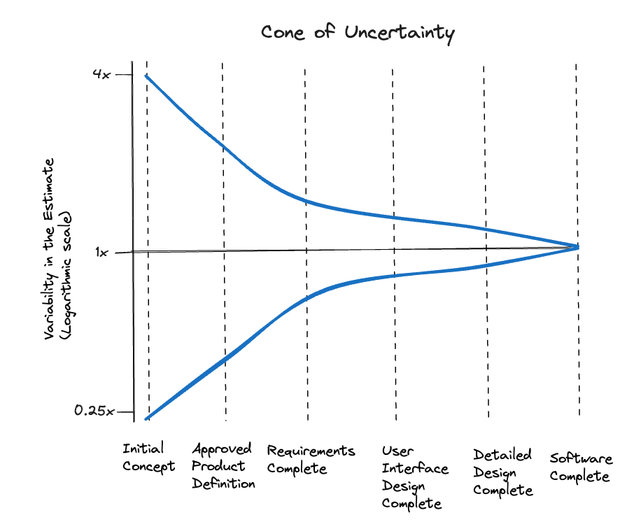
As the project’s information becomes more available, the variability narrows. It is important to note that the diagram represents a best-case scenario. In order to achieve this result, a proper business engineering is necessary. The study was based on classic waterfall projects. To use the milestones in my context, I mapped them to Scrum artifacts and ceremonies.
| Project Milestone | Agile Project Equivalent | Possible Error on Low Side | Possible Error on high Side | Range of High to Low Estimates |
|---|---|---|---|---|
| Initial Concept | Product Vision | 0.25x | 4x | 16x |
| Approved Product Definition | Backlog with Epics | 0.5x | 2x | 4x |
| Requirements Complete | Refined Stories | 0.67x | 1.5x | 2,25x |
| User Interface Complete | Sprint Planning I | 0.8x | 1.25x | 1.6x |
| Detailed Design Complete | Sprint Planning II | 0.9x | 1.10x | 1.2x |
By using this table, I can check if my estimation ranges match the volatility of the requirements at the specific phase of the software development process and adjust them. This often leads to ranges that are far wider than stakeholders are used to. Sticking to this result takes courage, but don’t worry; it gets easier with time. 😀
Estimation Tip #5
Consider the cone of uncertainty when choosing the estimation range.
The Distribution Function
We have seen that forecasts are communicated as ranges, but this is not very useful for planning. When to schedule trainings for a new software release for example, it is not possible to just say: “Dear colleagues, the training will take place between the first of May and the first of October according to the release date. Please be prepared and do not go on vacation. We will inform you as soon as possible.”
Making a plan requires discrete start and end dates for each task to map their dependencies. But what’s the best value to choose for the plan when you only have a range? By picking the lower boundary of the range, you’re taking a very high risk, but by selecting the maximum value on the other side, you’re losing the opportunity to release the software earlier and get a quick return on investment. Therefore, the consequences of missing a due date must be weighed against the profits of an early return on investment to find the sweet spot with the appropriate risk. For this decision, we need a correlation between the estimate values and their probabilities, or in more mathematical terms a probability distribution function.
Unfortunately there is no exact way to determine this function for the estimations we make, but we can choose a mathematical function to model it. The probably most known distribution function is the Gaussian Normal Distribution. This is how it looks for our estimation range:
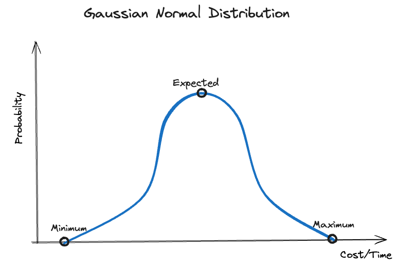
For each value, the graph shows the probability. The value with the highest probability lies in the middle of our estimation range and is called the expected value. We tend to choose this value for our plan intuitively, but this is quite risky. Despite having a 50% probability of the actual value being lower or equal to the expected value, there is also a 50% chance that the actual value is higher than the expected, meaning that the plan will not succeed. I don’t think this is what we are looking for most of the time, is it?
Software estimations present specific characteristics that make this situation even worse. In his book, McConnell suggests a more realistic distribution curve for software estimation than the Gaussian Distribution .
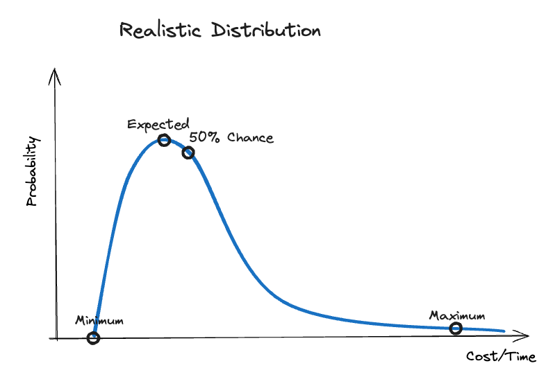
According to him, the chances of accomplishing a software task drop quite fast when we move from the expected to the minimum value. This is because there is a fixed value below which no one can accomplish the task. However, on the other side of increasing values, there are potentially endless options that can increase the actual effort. As a result, the curve drops much slower at higher values. There will always be situations where the estimated task cannot be completed, so it will never go to zero. As an example, the company’s goals can change and the project must be canceled. Our maximum value must therefore be one with a very low probability that we can ignore.
Because the curve is asymmetric, the expected value is no longer the value with a 50% chance, but rather lies just to the left of it. Moreover, there is another consequence that contributes to poor estimation results. When asked to provide an estimation range, we often start with the expected value and then consider the value we can achieve under perfect conditions as the minimum. Based on the Gaussian Distribution, we then assume that the maximum has the same distance to the expected value as the minimum. As shown in the following diagram, this misconception results in an unrealistically low maximum value.
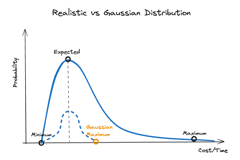
In order to avoid falling into this trap, ensure that you double check your maximum value if the expected value is just in the middle of your estimation range. It can be helpful to ask yourself: “Where is the value where I would quit my job when it is exceeded?” This is the real maximum even if it seems excessive. The next tip summarizes this strategy.
Estimation Tip #6
Choose a maximum that you are willing to pay a serious price when it is exceeded. Compared to the minimum on the other side, it should be farther from the expected value.
Let’s talk about Confidence
Let’s return to the question of which value to choose for planning. By deciding for the expected value, we leave ourselves with a chance for success of less than 50%, which is insufficient for most business plans. If we choose the maximum value, we are nearly 100% confident that our plan will succeed, but we risk sacrificing the chance of accomplishing the goal sooner. The value we are looking for is somewhere in between that represents the extent to which we are prepared to take the risk of failure. This value is called the confidence interval.
The question for the proper confidence interval must be addressed to the stakeholders who , ultimately, are taking the risks. For most of them, this is an unfamiliar request, so they struggle to respond. Using this diagram that illustrates a 90% confidence interval, I explain to them what I’m asking for.
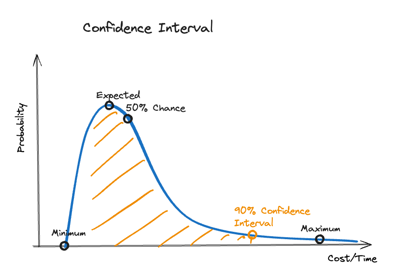
By analyzing this diagram, we can understand how the key elements of the estimation correlates to the chance of success.
- Minimum: It is impossible to accomplish anything below this value.
- Expected: This is the value with the highest probability, but also a chance to succeed of 50% in the best case.
- Confidence Interval: This value has a specified chance, that the actual value will be equal or less (for example 90% like in the diagram).
- Maximum: There is hardly a chance that the actual value will exceed this mark.
Instead of you making the decision for the stakeholders by providing just one of these values when asked for an estimation, they can use these data to determine the right value for their planning based on their willingness to take risks. This leads us to our final tip.
Estimation Tip #7
By providing expected value and confidence interval in addition to the estimation range, stakeholders can choose the appropriate value for their planning based on their risk affinity.
Conclusion
It has been shown that providing a single value as an estimation is not sufficient. In order to provide stakeholders with all information about risks, we must provide all of the key elements of an estimation: the minimum, the expected value, the confidence interval, and the maximum. A realistic distribution function and the cone of uncertainty must be respected to determine them reliably.
Now that we understand how estimations work, let’s examine how they are used in practice in the final part of this article series.